

It’s time again for 3 Google Sheets Formulas that will change your life. If you are a spreadsheet noob, make sure you hop over to How Do You Use Google Sheet Formulas to get a primer on this awesome functionality.
Ok, enough of the pleasantries. Let’s get to the good stuff.
I’ve got another 3 awesome formulas for you:
Formula 1: GOOGLE TRANSLATE
Scenario: You’re a teacher at a local public school. It’s time to send report cards home with grades and comments. Your school’s report card doesn’t translate anything to Spanish, so you’re stuck going to https://translate.google.com, to copy and paste your comments 1 by 1 to the translator, then copy and paste the translation back into your gradebook.

Ok, yeah that’s cool. But Forget that rubbish, head over to Google Sheets and enter the formula:
=googletranslate(text,[source_language],[target_language])
Let’s go through all the arguments here:
- Source_language = The language that you are starting with. Don’t type “English”, you’ll want to refer to this ISO list here: https://en.wikipedia.org/wiki/List_of_ISO_639-1_codes. In this case English = “es”
- Target_language = The language you’d like it to be translated to
- Text = the text you want to translate.
Putting the formula together:
You can either hard code your text into the formula like this
=googletranslate(“Hello, my name is Dr. Jay Aguda. What’s yours?”,”en”,”es”)
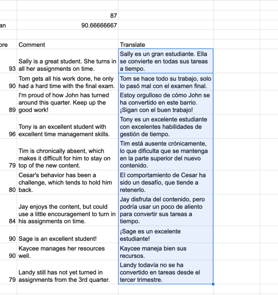
Or, back to that scenario, you’ve got a list of students with their comments: just refer back to the cell that contains the english comment then fill down!
=googletranslate(F3,”en”,”es”)
Formula 2: COUNT IF and COUNT IFS
Scenario: You’ve got a gradebook that not only contains grades, but also other demographics much like the sheet below.
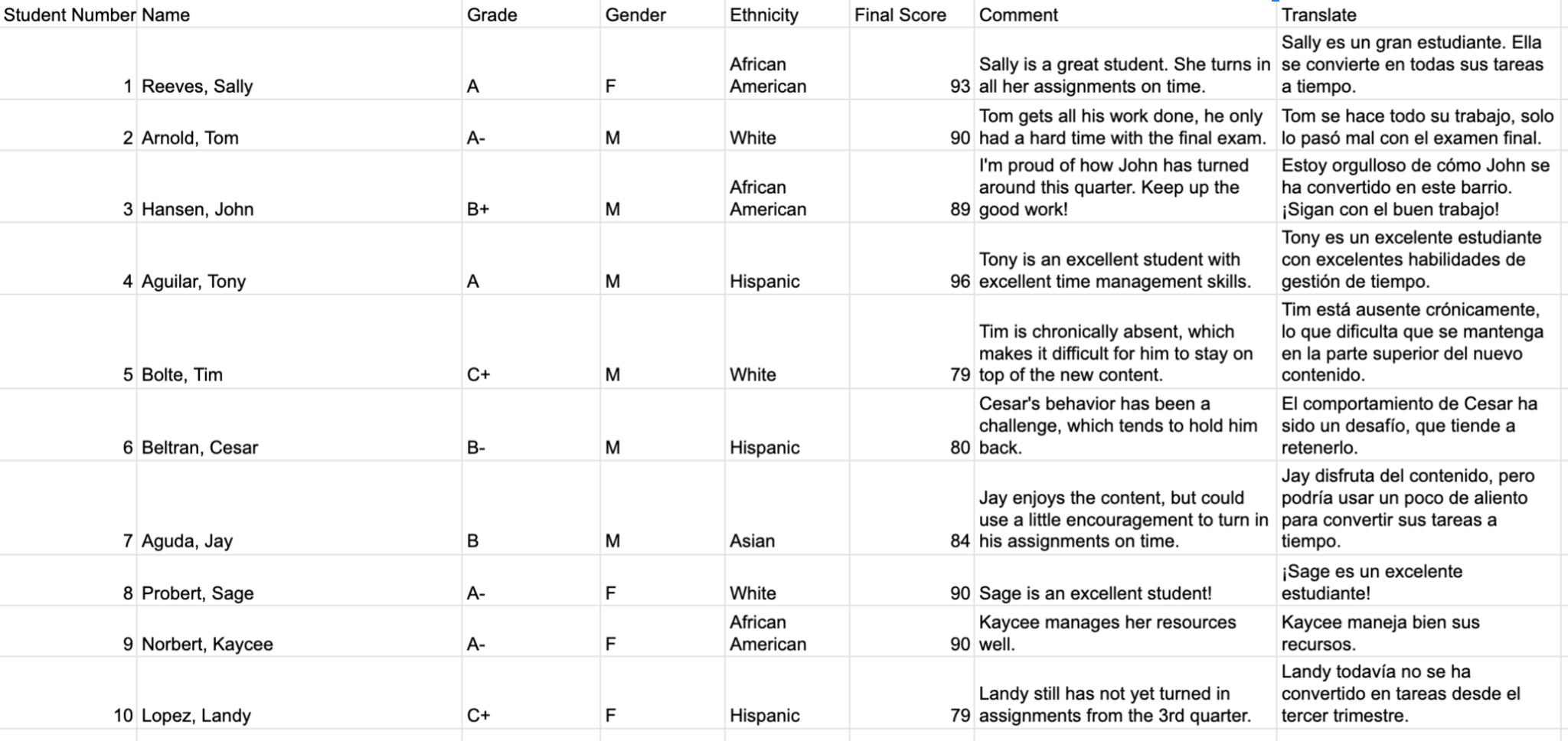
You want to count the number of students who are African American so that you can group them as a subgroup. Additionally, let’s say you’d like to get that broken down even further to see how many of those African American students are female.
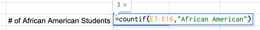
Use CountIF to count things in your list IF it meets a certain criteria
=COUNTIF(range,criteria)
Let’s break down the arguments here:
- Range: the range of data you are going to count – in the case below, I want to count the items in the E7 through E16 range)
- Criteria: tell google sheets to count only if they meet this criteria. You can write this, in this case, as “African American”. Sheets will only count items in this list that match “African American”
Wonderful! But now let’s get to the 2nd part of that scenario, what if you want Sheets to evaluate 2 different variables? Use COUNTIFS
=COUNTIFS(criteria_range1, criterion, criteria_range2, criterion2…)
Let’s break down the arguments here:
- Criteria_Range1: the range of data you are going to count for the FIRST criteria – in the case below, I want to count the items in the E7 through E16 range)
- Criterion1: tell google sheets to count only if they meet this criteria1. You can write this, in this case, as “African American”. Sheets will only count items in this list that match “African American”
As you can see, it’s basically the same. But in this case you can add as many criterion as you want. The more criterion, the longer your COUNTIFS formula will be. In this case, we are looking at 2 criterion. So:

Formula 3: AVERAGE and AVERAGEIF
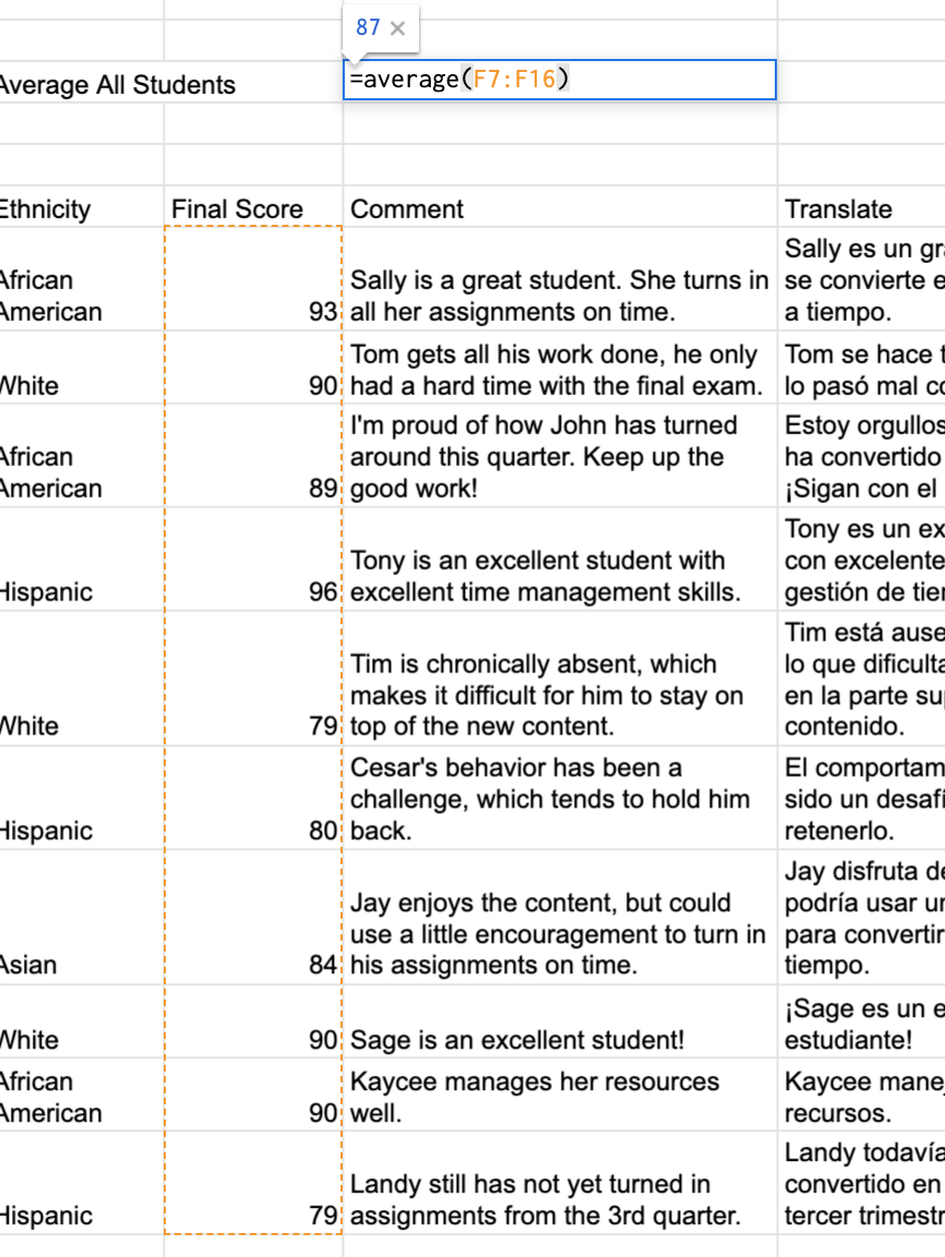
Scenario: You’d like the average score of all your students. You’d also like to see the average of your subgroup, African American students.
=AVERAGE(values)
Let’s break down the arguments here:
- Values: can either be a range or a comma separated list. In our case, because our data is in an entire uninterrupted column range, we’ll write it this way
Ok, so how about that subgroup? AVERAGEIF is your ticket here.
=AVERAGEIF(criteria_range,criterion,average_range)
Let’s break down this formula: You’ve got 3 arguments for this one:
- Criteria_range: the range that contains the data you are going to use to average only the things that match your criterion.
- Criterion: what you need to be in the criteria range so that the value is used in the average. In our example we are going to hard code “African American” so that only the items in the list that match “African American” will be included in the average.
- Average_range: the range of numeric values that you will use in your average calculation.

Now, go off and save some more time!